Note
This document describes general procedures to conduct manual observations with the Rubin Observatory Auxiliary Telescope. These procedures are influx and will evolve over time as the system matures, therefore it is highly recommended that users keep a close look on this document before doing any observations. Here we will also document troubleshooting to commonly found issues. In case of questions contact the document authors.
1 Introduction
It is important to emphasize that this document focus on early operations of the Auxiliary Telescope, with a significant part of the hardware and software still in need of considerable advancements. For instance, we are still in the process of obtaining and validating the telescope pointing model and optical alignment.
There is also some significant distinctions in the way we operate the telescope at this early stages and the way we plan to operate during commissioning and, even more, during normal operations. At this point we maintain a “low-level” kind of operations, both due to the need to be in full control of all the components and simply because the lack of high level operation software available. In fact, we are in the process of developing high level software that will improve considerably the user experience as well as pave the way for the development of “SAL Scripts” that ultimately will power the observatory Script Queue.
Furthermore, some issues pointed in this document may have been corrected in the meantime so it is very likely that the document will contain some outdated information. We will make an effort to document corrections as they occur but be aware that changes may happen faster then we are able to update this document. Users may want to check for more updated versions in the edition navigation page or check the github repository for any pending pull requests.
2 Network architecture and connectivity
From the user perspective, the summit network can broken down into two main systems; the campus and the control network. In principle, if you are at the summit, the base or in Tucson, if you are connected to the LSST network (e.g. LSST-WAP) you will have access to the summit network and the control network. IT managed to overlay both networks so that there is no need to use bastion hosts to access systems on the control network from LSST network. This considerably simplify user access to resources avoiding the need for ssh tunnels.
A list of the host computers IP addresses can be found here.
3 Monitoring and Interactive tools
Here is a list of currently available tools to monitor and interact with the system and a quick overview of how to use them. More details on how to perform specific tasks with the telescope are described furthermore.
3.1 Engineering and Facility Database (EFD)
The EFD is responsible for listening to and storing all data (Telemetry, Event, Commands and Acknowledgements) sent by components and users interacting with the components. The most recent incarnation of the EFD uses influxDB to store the data in a time-series database. See sqr-034 for details about the EFD implementation.
Data from the summit is available on chronograf and can be accessed at https://chronograf-summit-efd.lsst.codes/.
On the left hand side of the web page there is a tab with links to the different actions one can
perform with chronograf. Probably the two most useful tabs are Dashboards and
Explore; the first will take you to a list of available dashboards created by users that
gathers important information about the subsystems. The “Summary state monitor” is a good
example of general information one would be interested in during an observing night.
Important
The chronograf dashboards are shared between all users. If you feel like you need to make any change to the already existing dashboards, make sure to create a copy of the one you plan on editing and change that one instead.
The Explore tab let users perform free hand queries to the database using a sql-like
language.
In addition to the chronograf interface, users can also query for EFD data from Python using the efd-client library.
3.2 Jupyter Lab Servers
Jupyter notebooks are very popular amongst astronomers, specially in the LSST collaboration. They provide an easy and simple way of running Python code interactively through a web browser and give the additional benefit of combining documentation (using markdown language) and code. Users can run Jupyter notebook server locally on their own machine or on servers, enabling a cloud-like environment with access to powerful computing or, in the case of the LSST control system, to specialized functionality.
The most recent incarnation of Jupyter notebooks is Jupyter Labs. It provides access to a similar environment as that of a notebooks but with additional functionality.
We envision that Jupyter Lab servers will be a fundamental part of LSST control system, enabling users to perform low and high level operations in a well-known and interactive environment.
Important
As of 2020/01 the old user-based Jupyter Lab server is retired.
For that, users have access to a full-featured LSST Science Platform instance at the summit (LSP, [LDM-542]). Documentation about how to use the notebook aspect of the LSP can be found here.
Users will need to be registered in the rubin_summit_ops github organization to have access to the summit lsp instance. Once registered to that organization, open the LSST Science Platform instance at the summit and follow the users authorization instructions.
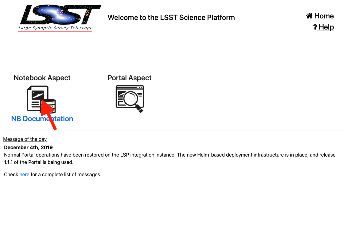
Once logged in, the user should see the welcome page page. Click in the icon bellow the “Notebook Aspect” (as indicated by the red arrow in the figure) and it will take you to the server spawning interface. Select an image on the left hand side (preferably the recommended one) and a computing resource size on the right hand. The image will dictate what lsst-stack software version will be available. All images ship with the running version of T&S communication libraries (ts_xml, ts_sal, ts_salobj and ts_idl). In terms of computing resources, it is usually recommended to select the Large type as operations notebook can be quite heavy. Then click on the start button and wait while the server is loaded.
Once the service is ready the page will be redirected to the jupyter lab interface.
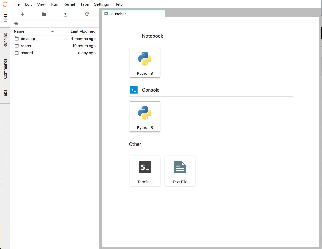
In the left hand there is a file browser navigation screen which, by default, have three directories;
develop, repos and shared. The develop directory is a bind mount on
the server that
runs the Jupyter Lab containers. Inside there is a repository for notebooks
(develop/ts_notebooks) with examples and work notebooks from other users (separated by
username). Feel free to browse and edit any notebook within this repo. Be sure to commit and push
any work you may have done and eventually make Pull Request to the original repo so other users can
see and use work that was done.
While each user has their only develop space, the containers have a shared mount space
visible to all users, shared. Filed placed or edited here by a user in their jupyter server
will be available/modified to all the other users.
The repos directory, on the other hand, contains some basic repos that ships with the
notebook server containing the T&S software used to power the control system. Any data in
this directory,
or in the home folder, will be lost if the container is restarted. It is advisable to only keep
important data inside the user designated folder (e.g. develop).
It is also possible to access data taken with the LATISS instrument in the notebook server.
The data is immediately available in a butler instance in
/mnt/dmcs/oods_butler_repo/repo/. This mount point is read-only by all users but
inside that there are a couple of shared mount places for users to save calibration
and reduced data (/mnt/dmcs/oods_butler_repo/repo/CALIB and
/mnt/dmcs/oods_butler_repo/repo/rerun).
3.3 LSST Operations and Visualization Environment (LOVE)
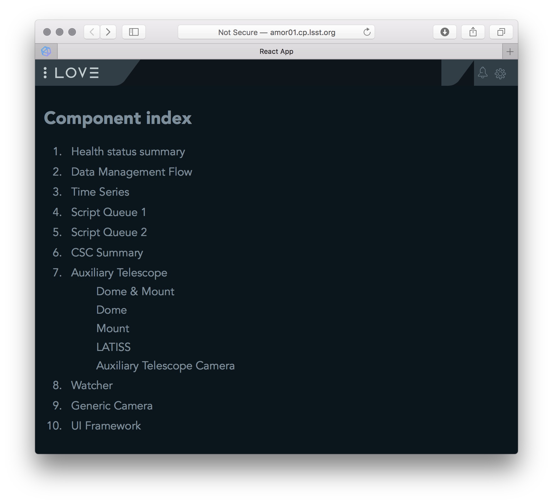
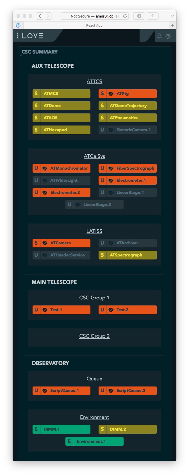
The LOVE interface is available at the summit on the following address; http://amor01.cp.lsst.org. In general, the interface will be visible in the observing room at the Summit and in Tucson. The current list of available views is influx, an example is shown bellow.
Note
The LOVE interface is still at a very early stage and users may experience some instabilities. Issues should be detailed in the observing log so developers can work on them afterwards.
3.4 Script Queue
Note
TBD
4 Auxiliary Telescope Commandable SAL Components (CSCs)
This diagram shows all the CSCs (light blue boxes) that are currently being used at the summit, their connections, the users jupyter servers and the salkafka producer that is responsible for capturing all SAL traffic, serialize it in avro an send it over to kafka to be inserted on the influx database (see sqr-034 for more information about the EFD).
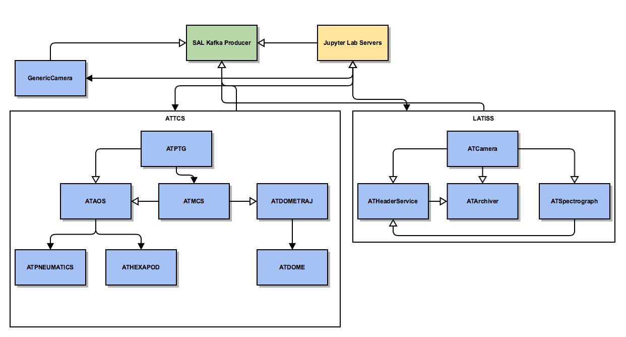
These components are grouped into high-level components that, although independent, work together logically. In the case of AT, these are the Auxiliary Telescope - Telescope Control System (ATTCS) and the LSST Auxiliary Telescope Image and Slit less Spectrograph (LATISS).
5 Basic Operations Procedures
This section explains how one can perform basic operations with the telescope using the Jupyter Lab server.
Note
Notebooks with the procedures can be found on the develop/ts_notebooks/examples
folder.
5.1 Startup procedure
At the end of the day, before observations starts, most telescope-related
CSCs will be unconfigured and
in STANDBY state. The first step in starting up the system is to enable all CSCs.
Putting a CSC in the ENABLED state requires the transition from STANDBY to
DISABLED and then from DISABLED to ENABLED. When transitioning from
STANDBY to DISABLED it is possible to provide a settingsToApply that selects
a configuration for the CSC. Some CSCs won’t need any settings while others will.
It is possible to check what are the available settings by looking at the settingVersions
event in the EFD, using Chronograf. Alternatively, it is also possible to let the high level
control scripts to decide which configuration to use. In most cases, when performing regular
operations, the auto-selection algorithm should be used.
To get started with it, make sure to open jupyter lab, navigate to the ~/develop/ts_notebooks/ folder nad create a directory with your username in that repository (e.g. tribeiro or pingraham). Then, navigate inside the newly created directory and create sub-directories as you see fit to keep the notebooks organized. Once you are happy with the location you selected for the nights operation start a clean notebook and enter the following to import the basic libraries.
import asyncio

from lsst.ts import salobj

from lsst.ts.standardscripts.auxtel.attcs import ATTCS
from lsst.ts.standardscripts.auxtel.latiss import LATISS
In the above, salobj is the high-level library that we use for basic
communication on component base. The following classes, ATTCS and LATISS
are developed using salobj to enable high-level operations combining multiple
components. The components involved in each of these high level classes are depicted
in the component diagram above.
It is possible now to use those classes to operate with the components. To enable them run;
domain = salobj.Domain()
attcs = ATTCS(domain)
latiss = LATISS(domain)

await asyncio.gather(attcs.start_task, latiss.start_task)

await attcs.enable()

await latiss.enable()
In case you want to enable the components with custom settings, it is possible to pass them as a dictionary, e.g.;
await attcs.enable(settings={
                'ataos': "current",
                'atmcs': "",
                'atptg': "",
                'atpneumatics': "",
                'athexapod': "current",
                'atdome': "test.yaml",
                'atdometrajectory': ""})
To prepare for the afternoon calibrations, run the high-level task.
await attcs.prepare_for_flatfield()
This method will position the dome and telescope to the appropriate position for taking
flat field data, open the mirror covers and all set up all other components to their
correct state. The LATISS class then offers high level tasks to acquire calibration
data.
bias_exp_id_list = await latiss.take_bias(nbias=10)

dark_exp_id_list = await latiss.take_darks(exptime=100., ndarks=10)

flat_exp_id_list = await latiss.take_flats(exptime=5., nflats=10,
                                           filter='blank_bk7_wg05',
                                           grating='ronchi90lpmm')
Each method will return a list of expId that allows users to access the data on a butler instance. We will give more details furthermore.
Once the calibrations are done and you are ready to open the telescope for the night, you can run;
await attcs.startup()
It is safe to run this method with the telescope in most states. The task will make sure to verify that all CSCs are in their proper state, will close the mirror covers before opening the dome and then proceed to open the dome and so on.
5.2 Pointing
The action of pointing and start tracking involves sending a command to the pointing component
(ATPtg) and then waiting for the telescope and dome to be in position while making sure
all components remain in ENABLED state.
When using the ATTCS class it is possible to perform the task with the following set of
commands:
import asyncio

import astropy.units as u
from astropy.time import Time
from astropy.coordinates import ICRS, Angle

from lsst.ts.standardscripts.auxtel.attcs import ATTCS
Initializing ATTCS class.
attcs = ATTCS()
await attcs.start_task
To slew the telescope and dome to a target, you should use the slew_icrs or slew_object task. Also, this will set the sky position angle (angle between y-axis and North) to be zero (or 180. if zero is not achievable).
The ATTCS class support slewing to a target using a Simbad-resolve name.
await attcs.slew_object(name="Alf Pav")
It is possible to use RA/Dec as hexagesimal strings or floats (and mix and match them). For instance,
await attcs.slew_icrs(ra="20:25:38.85705", dec="-56:44:06.3230", sky_pos=0., target_name="Alf Pav")
or
await attcs.slew_icrs(ra=20.42746, dec=-56.73508, sky_pos=0., target_name="Alf Pav")
It is also possible to slew to an RA/Dec target and request a rotator position. To do that use the
rot_pos argument instead of sky_pos. Note that this will request rot_pos at the
requested time, which will change as the telescope track the object.
await attcs.slew_icrs(ra="20:25:38.85705", dec="-56:44:06.3230", rot_pos=0., target_name="Alf Pav")
In addition, it is also possible to slew to an RA/Dec and request the rotator to be positioned
with respect to the parallactic angle. For that use the pa_ang argument instead.
await attcs.slew_icrs(ra="20:25:38.85705", dec="-56:44:06.3230", pa_ang=0., target_name="Alf Pav")
All rotator positioning strategies mentioned above are available in both slew_icrs and
slew_object methods.
The ATTCS class provides a couple different ways to execute offsets with the telescope; offsets in Az/El, RA/Dec and xy. These can be done with the following calls, respectively (all values are in arcsec);
await attcs.offset_azel(az=100., el=100.)

await attcs.offset_radec(ra=100., dec=100.)

await attcs.offset_xy(x=100., y=100.)
By default, the offsets are not cumulative meaning, executing the same command more than once, results in the same offset, e.g.;
await attcs.offset_azel(az=100., el=100.)
await attcs.offset_azel(az=100., el=100.)
is equivalent to
await attcs.offset_azel(az=100., el=100.)
It is possible to execute cumulative offsets using the persistent option in
the offset commands. Meaning;
await attcs.offset_azel(az=100., el=100., persistent=True)
await attcs.offset_azel(az=100., el=100., persistent=True)
is equivalent to
await attcs.offset_azel(az=200., el=200.)
5.3 Using the LSST Auxiliary Telescope Image and Slit less Spectrograph (LATISS)
Similarly to ATTCS, the LATISS class allow users to interact with the instrument in a seamless way, without the need to worry about most of the multiple components that form the instrument. It also makes an effort to facilitate data acquisition so users don’t have to worry about some details required by the system (like setting of specific values in commands).
We already went through the tasks available to acquire calibration data above. Let us now review the task to take object and engineering data and then how to access the data using the butler.
As with the calibration tasks, one can use the take_object and take_engtest tasks to get object and engineering test data respectively. These tasks are similar to that of take_flats where the user can specify a filter and grating in addition to an exposure time and number of exposures, e.g.;
object_data_id_list = await latiss.take_object(exptime=5., n=10,
                                               filter="blank_bk7_wg05",
                                               grating="ronchi90lpmm")

engtst_data_id_list = await latiss.take_engtest(exptime=5., n=10,
                                                filter="blank_bk7_wg05",
                                                grating="empty_1")
Again, the method will return a list of exposure ids that can be used to access the data on the butler.
from lsst.ip.isr.isrTask import IsrTask

import lsst.daf.persistence as dafPersist

dataPath = '/mnt/dmcs/oods_butler_repo/repo/'
butler = dafPersist.Butler(dataPath)

data_ref = butler.dataRef('raw', **dict(visit=object_data_id_list[0]))

exposure = isrTask.runDataRef(data_ref).exposure
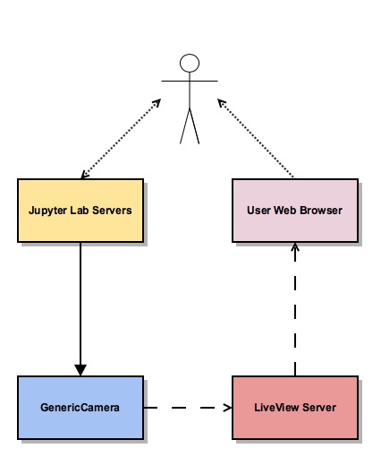
5.4 Using GenericCamera Liveview
The GenericCamera liveview mode can be used for quick look of telescope pointing, to check that a target is centered on the field after a slew was performed or to quickly evaluate the optics. When liveview mode is activated, the GenericCamera CSC will start a web server and start streaming the images taken with the selected exposure time. To visualize the images streamed by the CSC we created a separate web server that connects to the CSC stream and display the images. This is illustrated in the following diagram.
This is how to start live view in the GenericCamera;
from lsst.ts import salobj
import asyncio
d = salobj.Domain()
r = salobj.Remote(d, "GenericCamera", 1)
await r.start_task
Before starting live view, make sure to enable the CSC with the 4x4 binning settings.
await salobj.set_summary_state(r, salobj.State.ENABLED, settingsToApply="zwo_4x4.yaml")
When starting live view mode the user must specify the exposure time, which also sets the frame rate of the stream. So far, we have tested this with up to 0.25s exposure times.
await r.cmd_startLiveView.set_start(expTime=0.5)
Once live view has started, you should be able to access the live view server by
opening 139.229.162.114:8881 on a browser.
Attention
The web server that streams the live view data is not in a stable state. If the browser is not loading the page you may have to check the process running the live view server and restart it. Check the 6 Troubleshooting session for more information about how to restart it.
To stop live view, run the following command.
await r.cmd_stopLiveView.start(timeout=10)
5.5 Using GenericCamera to take (fits) images
The GenericCamera CSC was designed to emulate the same behaviour as that of the ATCamera and MTCamera CSCs. That means the commands and events have the same name and, as much as possible, the same payload and the events marking the different stages of image acquisition are also published at approximately the same stages.
To take an image with the GenericCamera first make sure that live view is not running. If live view is running the take image command will be rejected. Then, to take an image:
r.evt_endReadout.flush()
await r.cmd_takeImages.set_start(numImages=1,
                                 expTime=10.,
                                 shutter=True,
                                 imageSequenceName='alf_pav'
                                )

end_readout = await r.evt_endReadout.next(flush=False, timeout=5.)

print(end_readout.imageName)
You can download the image on your notebook server using the following command;
import wget
filename = wget.download(f"http://at-keener.cp.lsst.org:8000/{end_readout.imageName}.fits")
The command above will work as long as the user is connected to the LSST-WAP or equivalent network.
6 Troubleshooting
Here we describe some of the currently known issues and how to resolve them.
6.1 ATMCS won’t get out of FAULT State
Note
This issue has been resolved as far as we know. But, we’ll keep the issue and solution here in case it resurfaces.
In some situations the ATMCS will go to FAULT state and it will reject the standby command,
preventing to recover the system. We have been working on tracking this issue down but,
should you encounter this issue it is possible to recover by pressing the e-stop button on
the main cabinet (close to the telescope pier) and on the dome cabinet (east building wall on lower
level) and then executing the E-stop reset procedure. This should clear the FAULT state and leave the ATMCS in STANDBY.
6.2 Live view server is not responding
Note
This issue has been considerably mitigated and the live view server will be replaced soon by a view in the LOVE interface.
The live view server that is responsible for receiving images from the GenericCamera and streaming it to a user web browser is still in a very rough shape. The server connect to the GenericCamera over a TCP/IP socket and provides an image streaming server using a simple tornado web server. The connector that is responsible for receiving images from the CSC is still not capable of handling a dropped connection. That means, if there is a connection issue it is not capable of regenerating and continuing operations. Moreover, if the liveview mode is switched off on the CSC, the connection is also dropped and the live view server is also not capable of reconnecting.
If any of this happens the easiest solution is to restart the live view server. For that, you will need to connect to the container running the liveview server, kill the running procedure and restarting the process. This can be summarized as follows;
ssh liveview-host
docker attach gencam_lv_server
python liveview_server.py
Once the live view server is running you can detach from the container by doing Crtl+p Crtl+q.
6.3 Building CSC interfaces
Note
The latest notebook servers ships with the interfaces for all available components. These instructions are still useful in case you need to update the interface on the fly.
To communicate with a CSC, we use a class provided by salobj called Remote.
As you can see on previous sessions, the Remote receives the name of the CSC as
an argument, which ultimately, specifies the interface to load.
In order for the Remote to load this interface it needs to have the set of
idl libraries available. In some cases, the interface for the CSC that you plan
on communicating may no be readily available on the Jupyter notebook server. If
this is the case you will see an exception like the following when trying to
create the Remote.
---------------------------------------------------------------------------
RuntimeError                              Traceback (most recent call last)
<ipython-input-2-470a83f93eee> in <module>
----> 1 r = salobj.Remote(salobj.Domain(), "Component")

~/repos/ts_salobj/python/lsst/ts/salobj/remote.py in __init__(self, domain, name, index, readonly, include, exclude, evt_max_history, tel_max_history, start)
    137             raise TypeError(f"domain {domain!r} must be an lsst.ts.salobj.Domain")
    138
--> 139         salinfo = SalInfo(domain=domain, name=name, index=index)
    140         self.salinfo = salinfo
    141

~/repos/ts_salobj/python/lsst/ts/salobj/sal_info.py in __init__(self, domain, name, index)
    152         self.idl_loc = domain.idl_dir / f"sal_revCoded_{self.name}.idl"
    153         if not self.idl_loc.is_file():
--> 154             raise RuntimeError(f"Cannot find IDL file {self.idl_loc} for name={self.name!r}")
    155         self.parse_idl()
    156         self.ackcmd_type = ddsutil.get_dds_classes_from_idl(self.idl_loc, f"{self.name}::ackcmd")

RuntimeError: Cannot find IDL file /home/saluser/repos/ts_idl/idl/sal_revCoded_Component.idl for name='Component'
But, instead of Component it will be the name of the CSC you tried to connect to.
To resolve this issue, you will need to build the libraries. You can do that by putting the
following commands on a notebook cell:
%%script bash
make_idl_files.py <Component>
Again, you will need to replace <Component> by the name of the CSC.
7 Advanced Operations Procedures
This section explains advanced procedures which may be required, specifically during commissioning or during servicing.
7.1 E-stop Reset Procedure
If an E-stop has been activated (or possibly an L3 limit switch hit) then the following procedure must be followed to free the system. i
- Remove the issue that caused the E-stop to be activated.
- Activate both E-stops, the one on the telescope control cabinet, and the one on the dome control cabinet. Both will glow red.
- Release dome E-stop by turning clockwise a quarter turn or so
- Release main cabinet E-stop in the same manner
- Press the blue start button on the dome cabinet
- Press the blue start putton on the telescope control cabinet
If this is done correctly, all three LEDs on the Pilz devices in both cabinets should be brightly illuminated, as seen in the following image. If only the main cabinet is depressed, then only the top light is bright. If only the dome cabinet is pressed, the top and bottom lights are bright.
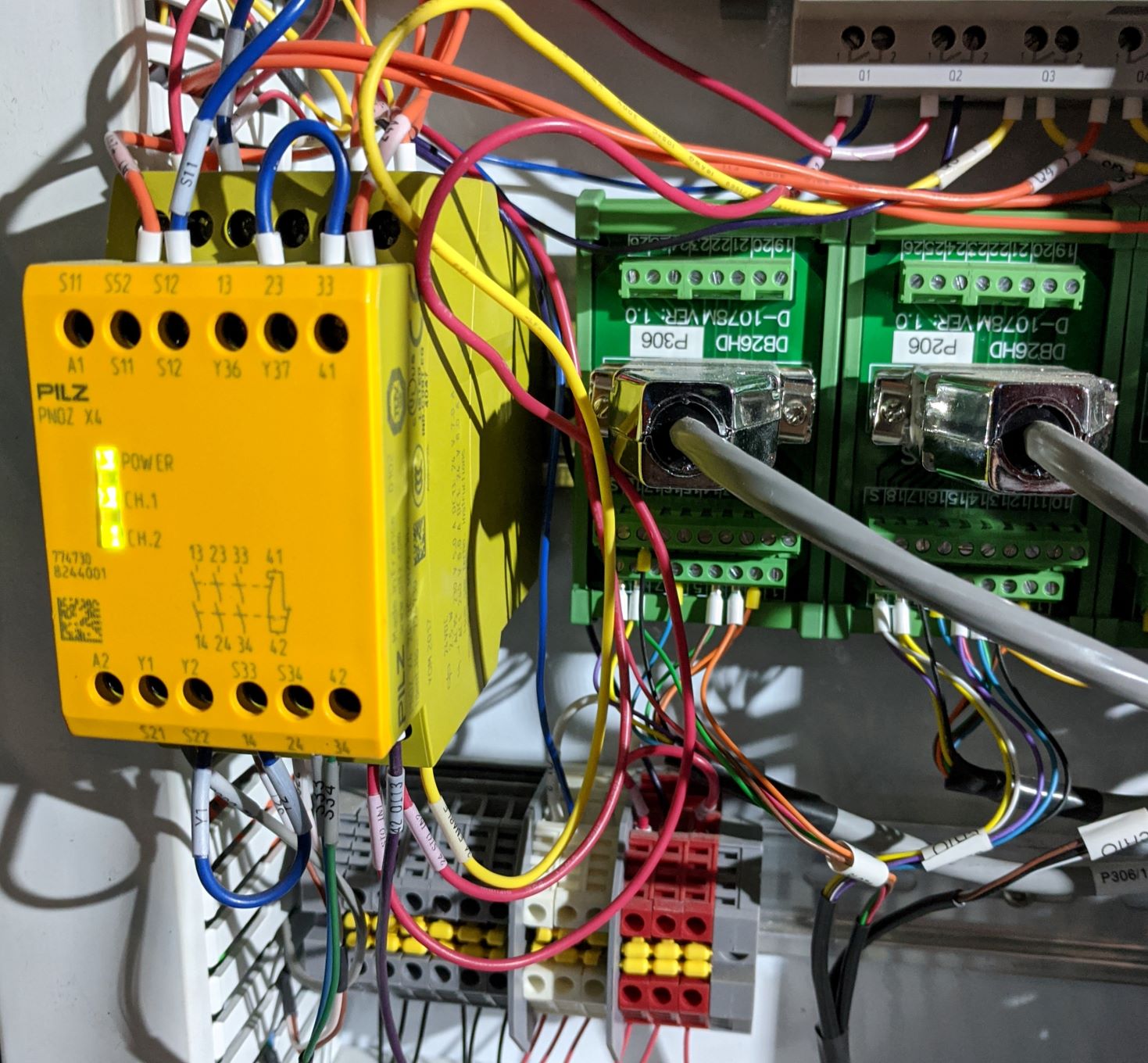
Figure 7 The Pilz controller in the Telescope Cabinet. All three lights illuminated means the E-stops are properly deactivated.
Note that if both E-stops are never activated simultaneously then the system will not reset.
Note
All L3 limit switches and E-stops are run through the smart relay system. This means that if an L3 limit (which is a hardstop at the extreme end of travel of the elevation, azimuth, M3 rotator and nasmyth axes) is contacted, then it will look as if an E-stop was pressed. To identify which L3 limit was hit, one must examine the interface of the smart relay. Any active signal will not have a filled box around the central number. The central number is then mapped to a L3 using the Auxiliary Telescope Electrical Diagram (Document-26731)
7.2 Viewing the ATMCS LabVIEW GUI
This is the GUI developed by Rolando Cantarutti and Omar Estay to display and interact with the telescope mount at a low-level (directly from the cRIO with no SAL communication). This is not meant to be used for regular operations.
Connections can currently be accomplished in two ways, the first uses a VNC connection to a windows machine currently located in the AuxTel building. The second is to login remotely using the LabVIEW Connector (requires Internet Explorer and a specific driver).
- Using RealVNC (which is required due to encryption although other clients
might work) connect to ‘atmcs-dev.cp.lsst.org’ on port 5900
Enter credentials (ask Patrick or Tiago)
- If the GUI is not already open, then open internet explorer and enter the
following address in the address bar.
http://atmcs-crio.cp.lsst.org:8000/atmcs.html
This machine is also connected to the ATDome and the ATSpectrograph low level controllers EUIs.
One can also install the LabVIEW remote panel on their Windows machine (Internet Explorer only) then open a tunnel to the above IP on port 8000. This requires the download from NI. Details will be included in the ATMCS documentation upon delivery. We don’t recommend this method unless absolutely necessary.
7.3 Resetting the ATHexapod IP Connection
Note
Outdated instructions. Needs updating.
For reasons which are under investigation, occasionally after a power cycle (we think) the hexapod TCP/IP connection goes down. To reset it, one must connect a serial port to the device, establish a connection using the (windows) PIMikroMove software, close the connection, then power cycle the controller. Power cycling can be done remotely (using the switched PDU). Until this problem is resolved, we’ve left a permanent serial (RS-232) connection to a local windows machine.
Follow these steps to re-establish TCP/IP connection:
- Establish VNC connection which is the same as the ATMCS GUI VNC shown here.
- Open PIMikroMove software from start menu
- Open new connection and select C-887 controller, and click connect
- Close connection
- Power cycle controller (which will cause the hexapod to lose the reference
- position)
- Put hexapod CSC in enabled state (which will send the hexapod to the
- reference position)
- Move hexapod to desired position
7.4 Mitutoyo Micrometers and Copley Controller Connections
The mitutoyo devices (when connected) are currently controlled through the Copley PC (located in the bottom of the telescope cabinet). Connection to this Windows machine uses TeamViewer. Contact Patrick for credentials.
More details to follow.
7.5 Telescope Cabinet Switchable PDU
Warning
DO NOT TRY THIS. This PDU server is where the camera ion pump and other critical components are connected. Unless you really known what you are doing, DO NOT TRY THIS.
In the event that a controller in the cabinet needs power cycling remotely, this may be done by logging into the switchable PDU mounted in the cabinet. The IP and connection info can be found here.
- Channel 1 is connected to the main 24V supply. This will power off the cRIO (and possibly the Copley controllers, Pilz Device, and Smart Relay).
- Channel 2 is connected to powerbar in bottom of cabinet, which has the 220V connection to the mount (which powers the Embedded PC for the Collimation Camera) as well as the hexapod connected to it.
7.6 AT Dome Communication Loss
If during operation the dome controllers lose connection, which is seen either from the software, or the push-buttons fail to work, then this procedure must be followed. The dome has two types of communication failsures
- The two cRIOs lose communication with each other (notably the cRIO in the
rotating part of the enclosure loses connection with the bottom box and may be
blocking the connection). If the CSC is connected and in disabled or enabled
state, then this will be shown in the scbLink event (must verify). Also, t
his can be seen in the Main Box Dome Control LabVIEW Remote on the ATMCS
machine as the TopComms light in the bottom left corner.
- Press the reset button on the cRIO inside the electrical cabinet on the rotating part of the dome (near the lower shutter) to resolve this issue
- The Main cRIO (located in the dome electrical cabinet on the first floor) is
not correctly releasing the TCP/IP connection. This can be observed by being
able to ping the box but not open a telnet connection (port 17310). Also,
the HostComms light will be illuminated in the Main Box Dome Control LabVIEW
remote.
- Press the reset button on the cRIO in the dome cabinet on the first floor to resolve this issue